BERT for Sentiment Analysis: How a Transformer Actually Reads

The previous post built image captioning with a CNN encoder and LSTM decoder. That was the pre-transformer world. This is what came next.

We fine-tuned BERT on movie reviews to classify sentiment, positive or negative. Simple task on the surface. But to understand why it works (and where it fails), you need to understand every layer. So let's go through it: tokenizer, embeddings, self-attention, multi-head, feed-forward, 12 encoder layers stacked on top of each other. No hand-waving.

---

What BERT Is

BERT is an encoder-only transformer. It doesn't generate text. It reads it and builds a context-aware representation of the input. Three stages:

1. Tokenizer + Positional Encoding: raw sentence → numeric vectors
2. Transformer Encoder: 12 layers of self-attention + feed-forward
3. Classification Head: CLS token → softmax → Positive/Negative

---

Stage 1: Tokenizer

The pretrained BertTokenizer does several things to your sentence:

1. Lowercase everything
2. Split by punctuation
3. Apply WordPiece: known words stay whole, unknown words split into subwords (e.g. "movie" stays as-is, an unknown word becomes "mo" + "##vie"). The ## prefix means "this is a continuation". No information about the split is lost.
4. Add special tokens: [CLS] at the start, [SEP] at the end
5. Convert tokens to integer IDs from the vocabulary

The tokenizer is pretrained. We don't touch it. We just use it.

---

Stage 2: Embeddings

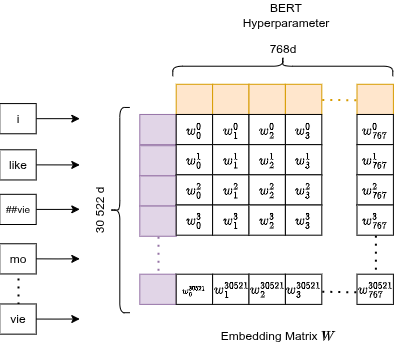
Token Embeddings

Each token ID gets mapped to a point in 768-dimensional space. That's the default BERT hyperparameter: 768 numbers per token.

This is just a learned lookup table (matrix of size vocab_size × 768). Mathematically, picking row 3185 is equivalent to multiplying the entire embedding matrix by a one-hot vector with a 1 at position 3185. A purely linear operation.

The embeddings are trained via backpropagation: when the gradient arrives here, it says "the vector for token X should shift in this direction." The optimizer (AdamW) updates that row directly.

Result: semantically similar tokens end up with nearby vectors in 768-d space.

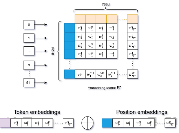
Positional Embeddings

Transformers have no notion of order. They process all tokens in parallel. To fix this, we generate a second set of embeddings for the position of each token (0, 1, 2, ...) and add them to the token embeddings.

Same mechanism: learned lookup table, same 768-d size. Position 0 gets its vector, position 1 gets its vector, and so on.

The combined embedding then goes through LayerNorm (stabilizes training) and Dropout (prevents overfitting).

---

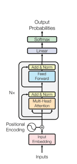
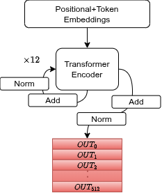
Stage 3: Transformer Encoder

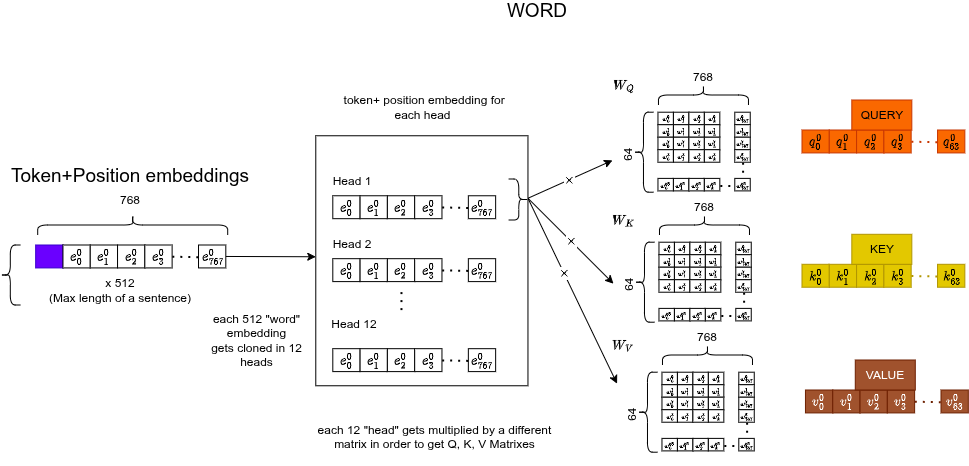
Q, K, V

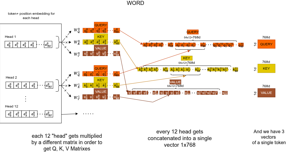
Each token's 768-d embedding gets multiplied by three separate learned weight matrices ($768 \times 64$), producing three 64-d vectors:

• Query $Q$: "what am I looking for?"
• Key $K$: "what do I offer as context?"
• Value $V$: "what information do I actually carry?"

e.g. Query: "I'm looking for a verb". Key: "I'm a subject". Value: "the word movie".

Here's the Q, K, V for a single token:

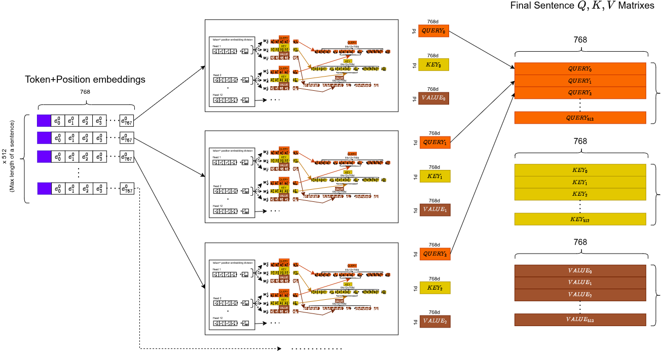
And across the full sequence:

The sentence-level view:

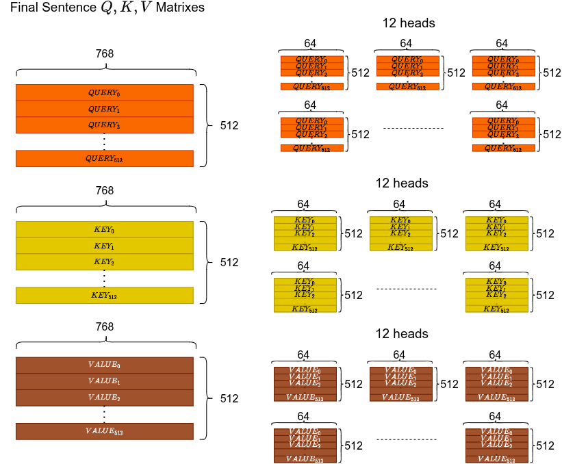
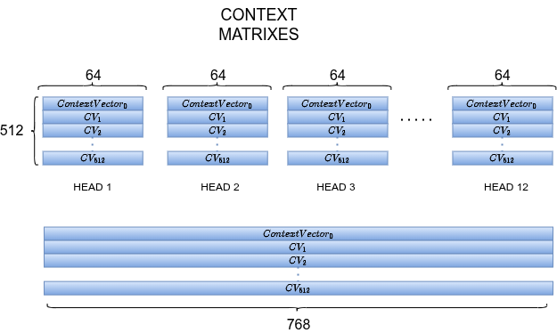
Multi-Head Attention (12 heads)

We don't do this once. We do it 12 times in parallel, each with different weight matrices. Each head specializes in a different "macro-sector" of understanding: grammar, coreference, synonyms, context, position, etc.

The model learns which heads specialize in what. Not hardcoded. Parallelization is a free side effect.

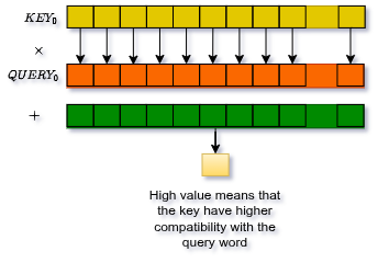
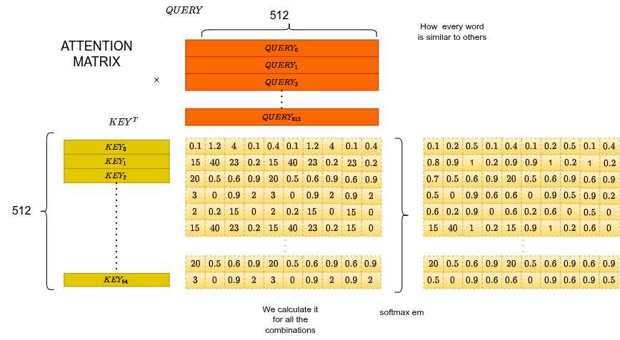
Attention Score

For each head, the attention score between token $i$ and token $j$ is the dot product of their query and key vectors:

$$\text{Attention}(Q,K,V)=\text{softmax}\left(\frac{Q\times K^T}{\sqrt{d_k}}\right)V$$

The $\sqrt{d_k}$ (square root of head dimension) scaling prevents the dot products from growing too large, which would push softmax into regions with near-zero gradients.

Why does $Q\times K^T$ work? If what a token is searching for (Query) and what another token offers (Key) point in the same direction, their dot product is high → high attention weight. If they point in opposite directions, near zero.

Classic example: the word "bank".

• $Quer{y}_{bank}$: "I need context. Am I money or nature?"
• $Ke{y}_{river}$: "I offer nature context"
• $Ke{y}_{city}$: "I offer institution context"

The high dot product between $Q_{bank}$ and $K_{river}$ resolves the ambiguity.

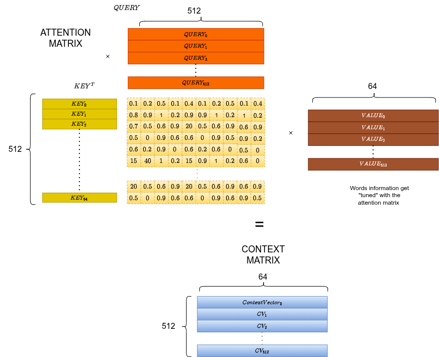
Attention Matrix

Apply softmax to the full $Q\times K^T$ matrix. Each row sums to 1. Row $i$ tells you how much each other token $j$ contributes to token $i$'s updated representation.

$$\text{softmax}(Q\times K^T)$$

Context Matrix

Multiply by $V$ to get the context-weighted representation:

$$\text{softmax}(Q\times K^T)V$$

Each row is now a token embedding enriched by attending to all other tokens.

Concatenation of All Heads

Each of the 12 heads produces its own context matrix (64-d per token). Concatenate all 12 → back to $12\times 64=768$ dimensions. Then pass through a final linear projection.

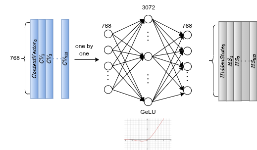
Feed-Forward Network

After attention, each token independently goes through a two-layer FFN:

$$768\stackrel{\text{Linear}}{\to }3072\stackrel{\text{GeLU}}{\to }3072\stackrel{\text{Linear}}{\to }768$$

The expansion (768 → 3072, 4×) amplifies patterns and lets the network combine features in a higher-dimensional space. GeLU introduces non-linearity with smoother gradients than ReLU. The compression brings it back to 768-d. Dropout prevents co-adaptation of neurons.

This is applied per token, independently. No cross-token interaction here, that was handled by attention.

12 Encoder Layers

The Attention + FFN block is repeated 12 times. Between each sub-layer: residual connection (input + output) and LayerNorm. The residual connections prevent gradient collapse through depth.

Dropout after attention, after FFN, and after embeddings throughout.

---

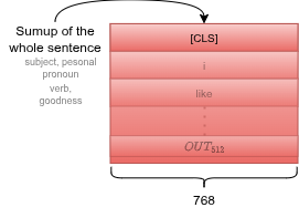
Stage 4: the CLS token

[CLS] is a special token prepended to every input sequence. It has no inherent meaning. It's a blank slate. But after 12 layers of self-attention, it has attended to every other token in the sequence. By the end of the encoder, the CLS embedding has aggregated the full semantic context of the sentence.

That's what we use for classification.

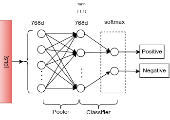
Classification Head

A pooler (a dense layer) transforms the CLS embedding (768-d) through tanh activation. Then a final linear layer maps it to 2 outputs (Positive / Negative). Softmax converts logits to probabilities.

$$768\stackrel{\text{Dense + tanh}}{\to }768\stackrel{\text{Linear}}{\to }2\stackrel{\text{softmax}}{\to }[p_{neg},p_{pos}]$$

---

Training

Dataset: IMDB Large Movie Review Dataset, 4,500 real reviews subsampled:

• 3,200 training samples (80%)
• 800 validation samples (20%)
• 500 test samples (held out)

Loss: Cross Entropy on the 2-class logits vs. true labels.

Backprop flow: error at the classifier head → pooler → 12 encoder layers → $W_Q,W_K,W_V$ and FFN weights updated at every layer → all the way back to the embedding lookup table.

We fine-tune the entire model, not just the head. Every weight adjusts.

---

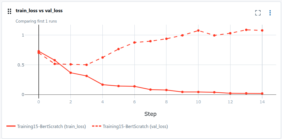
Overfitting and the Sarcasm Problem

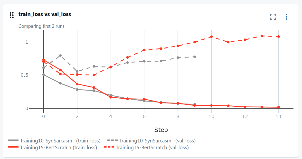
We trained for ~15 epochs. Around epoch 3, validation loss stops decreasing. The model overfits.

And there's a harder problem. The model fails completely on sarcasm:

"Great movie, if you enjoy watching paint dry for two hours." → classified Positive.

The model learned "Great" → positive signal, without understanding the ironic context that follows. This is a data problem, not a model problem.

---

Fix: Synthetic Data Generation

We generated synthetic sarcastic and ironic reviews using Qwen3 Instruct (Q4, running locally). The goal: teach the model that "Great" can be negative when followed by the right context.

The model still overfits, but validation performance improved. We still stop around epoch 3, but the decision boundary is sharper.

After adding synthetic data:

Input	Before	After
"Great movie, if you enjoy watching paint dry for two hours."	Positive	Negative
"The visual effects were stunning, but the plot made zero sense."	Positive	Negative
"I wish I knew what beautiful movie I just watched."	Positive	Negative

The third one is subtle. "I wish I knew" implies uncertainty and disappointment. The synthetic data pushed the model toward understanding that kind of inverted construction.

---

TL;DR

1. BertTokenizer: sentence → WordPiece subwords → integer IDs + [CLS]/[SEP]
2. Token + Positional embeddings: IDs → 768-d vectors, summed, LayerNorm + Dropout
3. 12 × (Multi-Head Attention + FFN): each token attends to all others, 12 heads specialize, $\text{softmax}(Q{K}^T/\sqrt{d_k})V$ is the core operation
4. CLS token aggregates full sentence context after 12 encoder layers
5. Classifier head: pooler + tanh + linear → 2 logits → softmax
6. Overfits after epoch 3 on IMDB. Sarcasm is the hard case.
7. Synthetic data from a local LLM fixes the sarcasm failure mode