CNN + LSTM Image Captioning: No Transformers, No Vibes, Just Math

Look, I get it. It's 2026, everyone's using ViT + GPT-4o to caption images in two lines of Python. But here's the thing: if you don't understand the pre-transformer era pipelines, you don't actually understand what's happening inside the modern ones. The attention mechanism is just a better version of what we're about to describe.

So we built an image captioning system from scratch. ResNet50 as the encoder, LSTM as the decoder, trained on Flickr8k. No pretrained language models. No CLIP embeddings. Just convolutions, matrix multiplications, and gated memory cells. Let's go.

Architecture in one sentence

A CNN encoder (ResNet50) extracts spatial features from an image and compresses them into a 256-d vector. A LSTM decoder takes that vector and generates a caption, word by word.

Encoder output concatenated with embedded captions, fed into an LSTM to generate the related sentence. That's it. Everything else is implementation. Let's peel the layers.

Part 1: Convolution

Take an image $I$ made of black and white pixels. You can write the intensity as numbers. Each cube below is a number from 0 to 255.

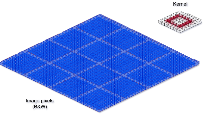
Black and white image as a 3D grid of pixel values, with a kernel overlay in the top-right corner

Define a kernel $K$ as a small $m \times n$ matrix of learnable weights used to extract features from the image.

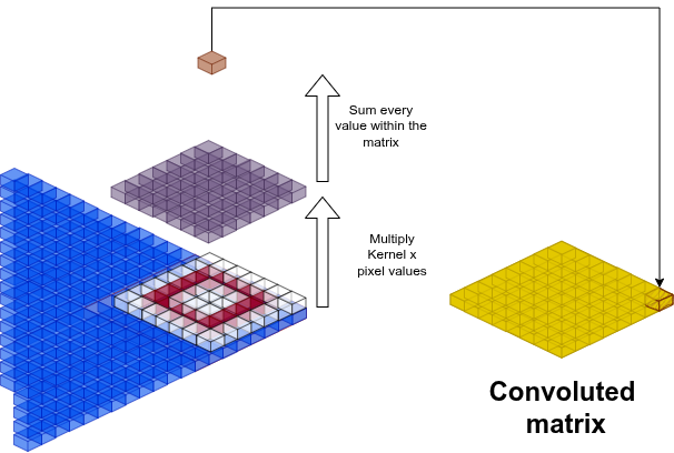
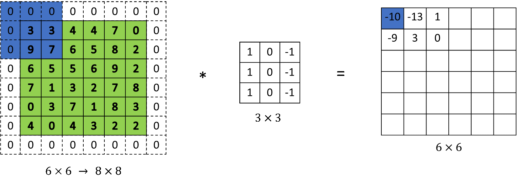
A convolution is a linear combination $S$ between image pixels and one or more filters:

$S (i, j) = (I * K) (i, j) = m \sum n \sum I (i - m, j - n) \cdot K (m, n)$

$i, j$ are the output coordinates in the convolved matrix. The result is one cell of a new, smaller matrix: the feature map. The kernel extracts local patterns: edges, gradients, corners.

Convolution sliding a kernel across a pixel grid, producing a feature map

Stride and Padding

Stride $S$ : how many pixels the kernel moves per step
Padding $P$ : zero-pad the border to control output size

Given image $M \times M$ and kernel $K \times K$ , output size is:

$O = \frac{M - K + 2 P}{S} + 1$

Stride and padding visualization on a convolution grid

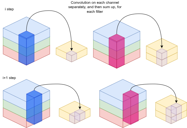
Color images: 3 channels

For RGB, you run the kernel across each channel (R, G, B) separately, then sum:

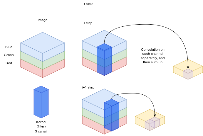
$S (i, j) = c = 1 \sum 3 (u = - h \sum h v = - w \sum w I (i - u, j - v, c) \cdot K (u, v))$

3D convolution on a color image — same filter applied to each RGB channel, results summed

By adding more filters, you get more channels (features) to explain the image.

Multiple filters producing multiple output feature channels

The whole point of a CNN is to transform an image into a vector of features.

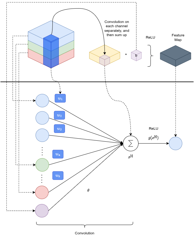
Convolutional Layer

Take the feature matrix from the convolution (linear operation), add a bias, apply ReLU (non-linear). It's like a neural network where the input nodes are the channel intensities under the kernel, the weights are the kernel values. The bias prevents the function from being forced through the origin, letting the network represent patterns with an offset.

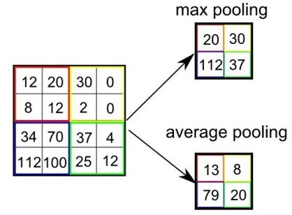
Convolutional layer: convolution output + bias → ReLU activation → feature map

Pooling Layer

Max pooling picks the max in each window. Average pooling averages. Both reduce spatial dimensions, aggregate features, and directly suppress overfitting.

Max pooling vs average pooling on a feature map grid

Part 2: ResNet50, the encoder

ResNet50 is our feature extraction backbone. It transforms input images into meaningful feature representations through an initial stage + four residual block stages. In the final flattening stage, we strip the classification head to preserve feature maps instead of producing class predictions.

Why "Res"?

"ResNet" stands for Residual Network. The core idea: instead of learning a full mapping, layers learn the residual: the difference between input and desired output. A skip connection bypasses one or more layers and adds the original input directly to the output.

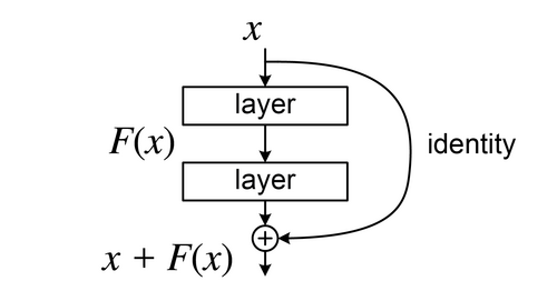
Residual block diagram: output = x + F(x), skip connection bypassing two layers

Gradients flow directly through the skip connection during backprop. This solves the vanishing gradient problem and makes it practical to train 50+ layer networks.

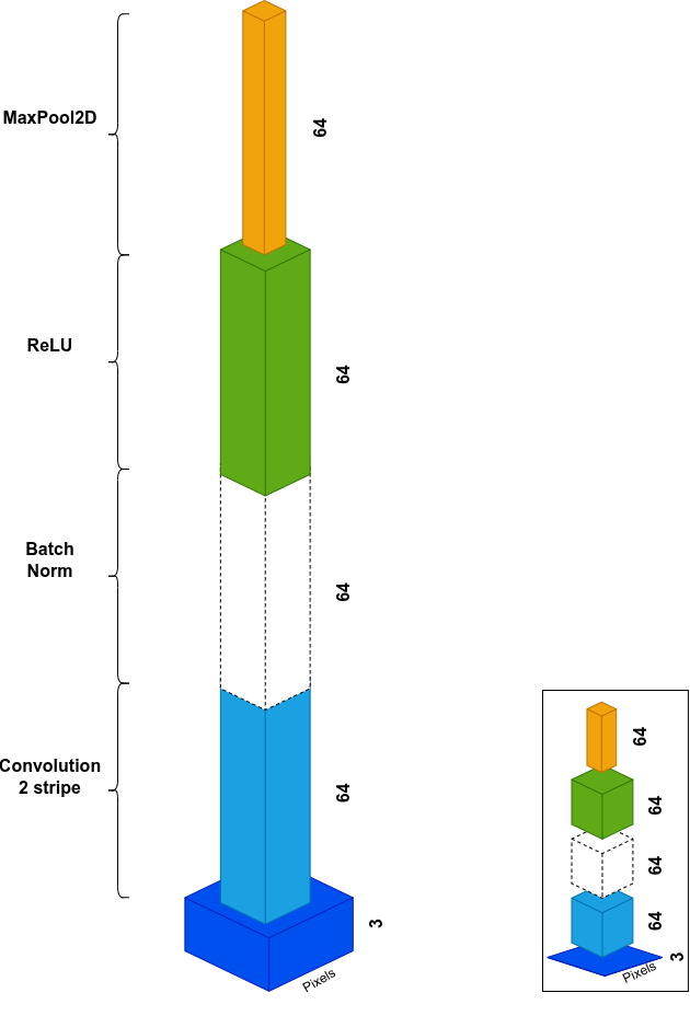
Initial Stage

7×7 Conv, stride 2 → halves spatial resolution, removes pixel noise
BatchNorm → mean 0, variance 1, stabilizes gradients
ReLU → non-linearity, zeros out negatives
3×3 MaxPool, stride 2 → another 2× downsample, adds translation invariance (small shifts don't change the max, features stay robust)

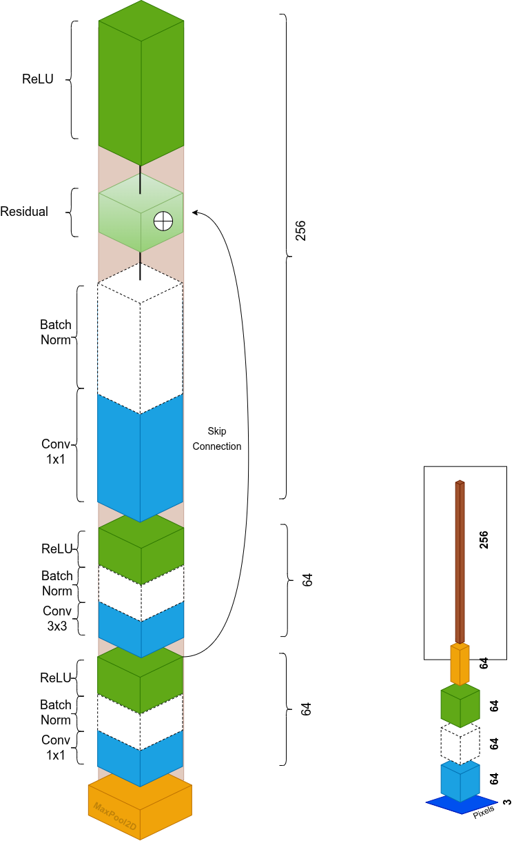
ResNet50 initial stage: aggressive spatial reduction from raw image to 64-channel feature maps

Bottleneck Residual Blocks

Each residual block has 3 convolutions, the bottleneck design:

Step	Operation	Purpose
1	1×1 Conv	Reduce channels (compress computation)
2	3×3 Conv	Extract spatial context
3	1×1 Conv	Restore/expand dimensions

The skip connection adds the original input to the output. When dimensions don't match (e.g., 64 → 256), a 1×1 conv on the skip path handles the projection.

First bottleneck block: 1×1 → 3×3 → 1×1 convolutions with skip connection, repeated 3 times

After the first stage, each new stage increases semantic complexity by trading spatial resolution for channel depth. The 3×3 conv uses stride=2 to halve spatial dimensions while extracting spatial features:

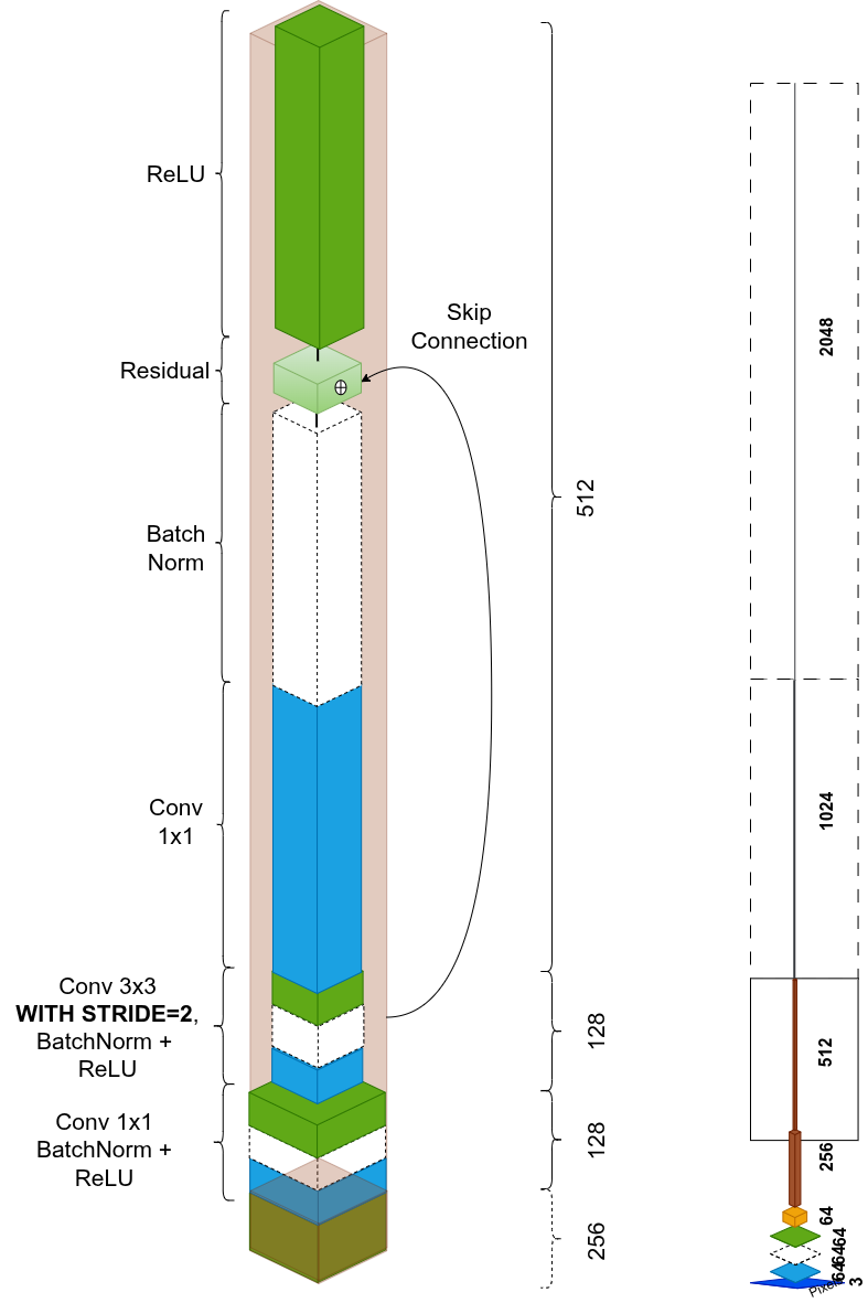
Subsequent bottleneck stages: stride=2 on 3×3 conv, channels grow 256 → 512 → 1024 → 2048

Stage repetitions, experimentally found optimal: 3 → 4 → 6 → 3 blocks. Final output: 2048 channels at 7×7.

Flattening Stage

After 2048 channels at 7×7, ResNet does a final compression:

Adaptive Average Pooling: collapses all 49 spatial pixels (7×7) into a single value per channel through averaging. Keeps only semantic essence.
Linear projection: converts feature space from 2048 to 256:

$256 \times 1 y = 256 \times 2048 W \cdot 2048 \times 1 x + 256 \times 1 b$

BatchNorm: normalizes the embedding for stable distance metrics.

Result: a compact 256-dimensional fingerprint of the image.

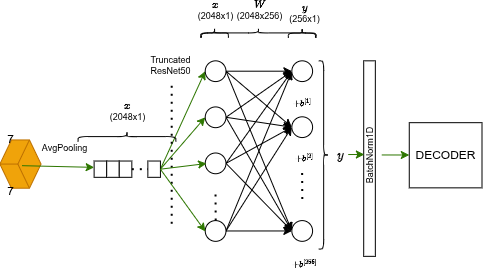
Flattening stage: adaptive avg pooling → linear projection 2048→256 → BatchNorm → 256-d vector

This final embedding feeds the LSTM decoder.

Part 3: Decoder

Vocabulary

Words with frequency < 5 are discarded. Special tokens added: <PAD> (padding to equalize sequence lengths), <START>, <END>, <UNK> (unknown for discarded words). Final vocabulary: 5,507 words.

Embedding Layer

A trainable lookup table: matrix $W$ of size $5507 \times 256$ .

Each word maps to an integer index → a row of $W$ . The embedding is trained end-to-end, so semantically similar words ("dog", "cat") end up with nearby vectors in 256-d space.

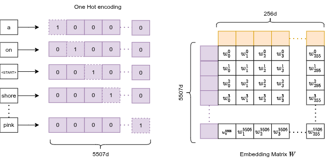
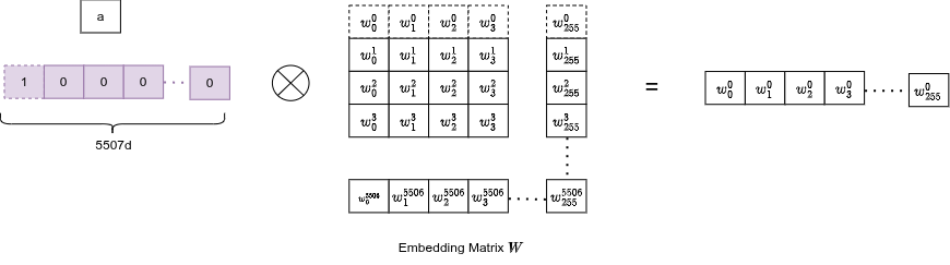
Embedding lookup table: word index → row of 5507×256 matrix → 256-d word vector

Since words are one-hot encoded internally, the matrix multiplication collapses to a simple row lookup: the exact row of the embedding matrix gets selected:

Embedding selection: one-hot encoded word picks the exact row from the embedding matrix

Concatenation

The image vector acts as the first token at $t = 0$ . Word embeddings follow in sequence:

sequence = [image_vec | word_0 | word_1 | ... | word_T]

Image features act as the initial input, followed by the word embeddings. This is what feeds the LSTM.

Part 4: LSTM

We use Long Short-Term Memory instead of a vanilla RNN for two reasons:

The model must remember the image (seen at $t=0$) all the way to the end of the sentence. That requires long-term memory.
LSTMs mitigate vanishing gradients on long sequences via gate structure.

Two states travel through time:

Hidden state $h_{t}$ (256-d): short-term memory, visible output, used to predict the next word
Cell state $C_{t}$ (256-d): long-term memory highway that carries crucial info (e.g., the image subject) without degrading

At $t = 0$ , states are initialized to zero and the image vector is the first input.

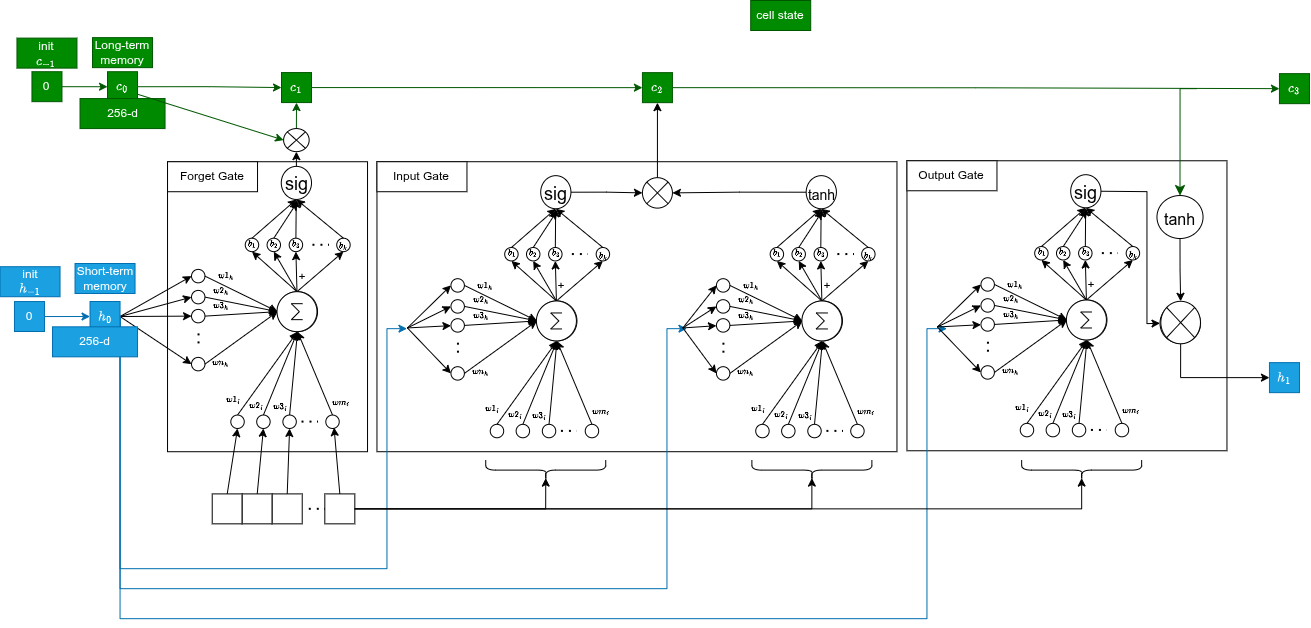
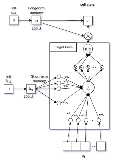
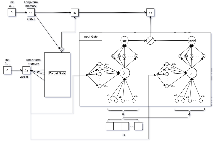
LSTM general architecture: cell state and hidden state flowing through time, with gate operations at each step

Forget Gate

Decides which information from past memory ($C_{t-1}$) is no longer needed.

Looks at current input $x_{t}$ and previous hidden state $h_{t - 1}$ , multiplies each by weights, sums, adds bias, passes through sigmoid:

$f_{t} = σ (W_{k} \cdot h_{t - 1} + W_{n} \cdot x_{t} + b)$

Output: values 0 (forget) → 1 (keep) for each element of the cell state.

After outputting "man", the gate might forget the generic "subject exists" feature to free memory for tracking the verb.

Forget gate: sigmoid output masks the previous cell state element-wise

Input Gate

In parallel, decides what new information to write into long-term memory.

tanh network → candidate values $\tilde{C}_{t}$ (range −1 to +1, e.g. singular/plural feature intensity)
sigmoid network → how important is each candidate (0 to 1)

Multiply both, add to the gated previous memory:

$C_{t} = f_{t} \cdot C_{t - 1} + tanh (\cdot) * σ (\cdot)$

Old memory is updated: forget the old, add the new weighted by importance.

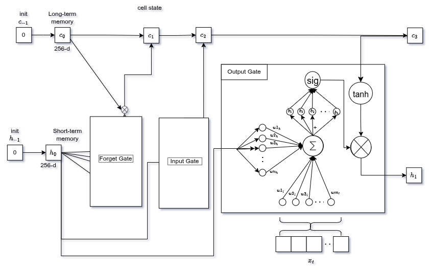
Input gate: tanh candidates × sigmoid filter added to gated previous cell state

Output Gate

Decides what the next hidden state (short-term memory) should be.

sigmoid decides what parts of the cell state to output. Then $C_{t}$ goes through tanh (push values to −1 to +1) and gets multiplied by the sigmoid output:

$h_{t} = σ (\cdot) * tanh (C_{t})$

The memory knows the subject is "singular cat", but if we need to predict a verb, the output gate filters out only the "singular" information to conjugate correctly.

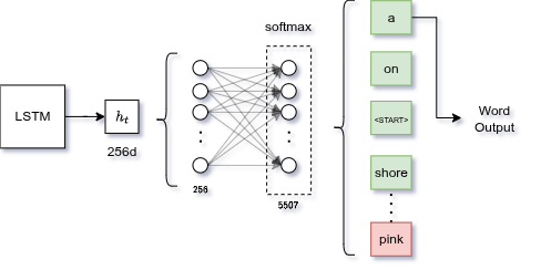
Output gate: sigmoid filter × tanh(cell state) = new hidden state

Final Fully Connected Layer

LSTM output $h_{t}$ (256-d) is an abstract concept. We need to translate it into an actual vocabulary word.

Linear layer: weight matrix $256 \times 5507$ projects hidden state onto a vocabulary-sized vector.

Training: Cross Entropy Loss comparing logits against the real next word (teacher forcing: feed the real word at time $t$ as input for step $t+1$)
Inference: pass logits through softmax, pick highest-probability word, feed it back as next input

FC layer: h_t (256-d) → linear 256×5507 → softmax → word probability distribution

Training

Dataset: Flickr8k: 8,000 images, 5 captions each = 40,000 pairs.

Strategy: Teacher forcing. Feed the real caption word at time $t$ as input for step $t + 1$ . Forces the model to learn correct predictions rather than compounding its own errors during training.

Data augmentation per epoch to force learning of robust visual concepts:

Random crop and resize
Horizontal flip
Color jitter (brightness/contrast)
Slight rotations

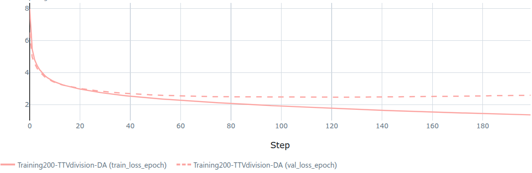
Results

Training loss decreased steadily. Validation loss stabilized around epoch ~150, then slightly increased. Mild overfitting.

Training vs validation loss over 200 epochs — validation plateaus around epoch 150

Output example 1

Output example 2

Output example 3

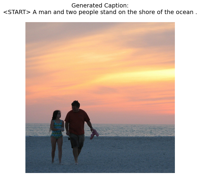
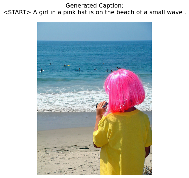
Subjects, actions, and settings are correctly identified. Syntactically a bit rough. Semantically reasonable though. Not bad for zero pretrained language model.

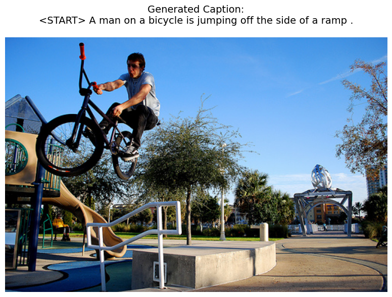
The Architectural Bottleneck

Here's the flaw: all visual information must pass through a single 256-d vector. By word 5, the model is generating "bicycle" but the image encoding is diluted across everything the ResNet ever saw.

Attention mechanisms fix this: instead of a single summary vector, the decoder can query the spatial feature maps from ResNet (7×7 × 2048) at each step, attending to the relevant image region. The model asks "what part of the image is relevant right now?" That's the next step.

TL;DR

ResNet50: image → 256-d vector (convolutions + residual blocks + adaptive pooling + linear projection)
Embedding layer: words → 256-d vectors (trained end-to-end, semantically meaningful)
LSTM: [image, word_0, word_1...] → next-word distribution (3 gated memory operations per step)
Cross entropy loss + teacher forcing during training
Slight overfitting after epoch 150, outputs are coherent
Single vector bottleneck is the architectural flaw → attention is the fix