MLP from Scratch: 98% Accuracy on Cancer Classification, No Keras Required

Before you reach for PyTorch, you should understand what you're reaching for. So we built an MLP from scratch. Raw Python, no autograd, no framework magic. We ran it on a real binary classification problem: detecting malignant vs. benign breast cancer tumors. 569 samples, 30 features, 20 hyperparameter configurations. Let's go through it.

Why MLP instead of logistic regression

Logistic regression works. But it's linear. When your hypothesis has non-linearities, you have two options: manually engineer polynomial features (which explodes your feature space fast), or let the network learn those non-linear representations for you.

An MLP is the second option. It learns non-linear combinations of inputs by stacking layers of neurons, each applying a non-linear activation. No feature engineering needed.

Perceptron vs Multi-Layer Perceptron: from a single neuron to a layered network

The artificial neuron

Each neuron takes $K$ inputs and a set of weights, computes a weighted sum, and passes it through an activation function:

$x = k \in K \sum W_{k} \cdot y_{k}$

$Y = f (x)$

The weights $W_{k}$ determine how much attention the neuron gives to each input. Different neurons in the same layer learn different weight distributions, building different representations of the same data. That's how the network can capture multiple patterns simultaneously.

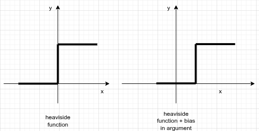
Why you need a bias

Take the Heaviside step function as your activation. If the weighted sum is exactly 0, the neuron outputs nothing and learns nothing. You fix this by adding a constant bias term to the linear combination:

$Y = f (k \in K \sum (W_{k} \cdot y_{k}) + 1)$

The bias shifts the activation function horizontally, letting the neuron fire even when the inputs alone don't push the sum above zero.

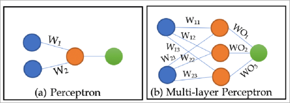
Heaviside function without bias (left) vs with bias (right): the curve shifts along the x-axis

Architecture

Stack enough neurons in a layer and you get more representational capacity. Stack layers and you get hierarchical representations. An MLP is a fully connected feed-forward network: every neuron in layer $i$ connects to every neuron in layer $i + 1$ .

MLP architecture: input layer, hidden layer, output layer, all fully connected

For this project: 30 input features, one hidden layer (we sweep the size), one output neuron. Sigmoid activation throughout because this is binary classification.

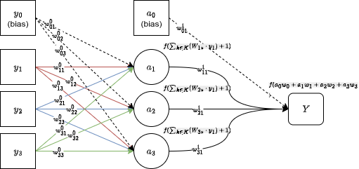
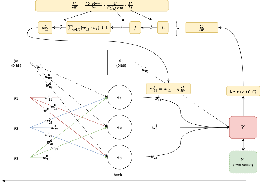
Forward propagation

You push the inputs forward through the network, computing the linear combination and activation at each layer, until you reach the output $Y$ .

$Y = f (k \sum a_{k} w_{k}^{1} + 1) where each a_{k} = f (j \sum y_{j} w_{j k}^{0} + 1)$

Forward pass: inputs flow through hidden layer activations to produce the output prediction Y

The output $Y$ is your prediction. Now you need to compare it against the real label $Y^{'}$ and compute an error $L$ .

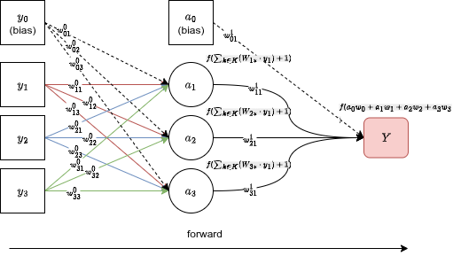
Backpropagation

Backprop is the chain rule applied to a computation graph. You have a loss $L$ (error between $Y$ and $Y'$), and you want to know how much each weight contributed to that error, so you can update it in the right direction.

To get $\frac{\partial L}{\partial W}$ for a weight in layer $i - 1$ , you walk backward through the computation graph, chaining gradients at each step:

$\frac{\partial L}{\partial W} = \frac{\partial \sum _{K} ( w \cdot a )}{\partial w} \cdot \frac{\partial f}{\partial \sum _{K} ( w \cdot a )} \cdot \frac{\partial L}{\partial f}$

Once you have the gradient, you update the weight proportionally:

$w_{11}^{1} \leftarrow w_{11}^{1} - η \cdot \frac{\partial L}{\partial W}$

Where $η$ is the learning rate. This is gradient descent.

Backpropagation: chain rule flows backward through the network, updating every weight proportionally to its contribution to the error

The dataset

Breast Cancer Wisconsin (Diagnostic) from UCI/Kaggle.

569 instances, 30 numerical features
Classes: malignant (212 samples, 37.3%) vs benign (357 samples, 62.7%)
Features: per-cell-nucleus measurements (radius, texture, perimeter, area, smoothness, compactness, concavity, symmetry, fractal dimension). Mean, standard error, and worst value of each.

The class imbalance (62/38 split) is mild enough that you don't need oversampling, but you do need to track both precision and recall, not just accuracy.

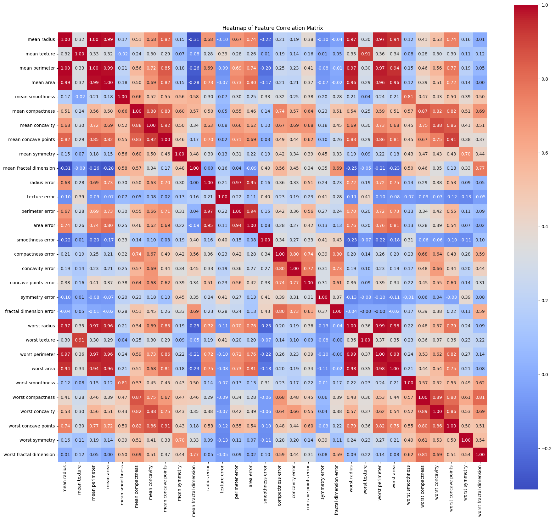
Feature correlation heatmap: some features are heavily correlated, e.g. radius, perimeter, and area are nearly identical

The heatmap makes something obvious: radius, perimeter, and area are almost perfectly correlated. You're feeding the network redundant features, but an MLP can handle that. It'll just learn to weight them accordingly.

Standardization

The features have wildly different ranges. Mean area goes from 143 to 2501. Mean smoothness goes from 0.053 to 0.163. If you don't normalize, the weight updates during gradient descent will be dominated by the high-range features.

Fix: standardize every feature to mean=0, variance=1.

$z = \frac{x _{i} - μ}{σ}$

We used StandardScaler from sklearn. One line, no reason to rewrite it.

Grid search

We ran 20 configurations: 5 hidden layer sizes × 4 learning rates.

Hidden neurons: 2, 5, 15, 30, 50
Learning rates: 0.01, 0.1, 0.50, 1.5
Max epochs: 200
Early stopping: if avg validation loss exceeds the minimum validation loss 10 times in a row, stop

The early stopping is important. Without it, you'd run all 200 epochs every time and waste compute on configurations that clearly stopped improving at epoch 15.

Results

Config	Hidden	LR	Epochs	Val Loss	Test Acc
MLP_H30_LR1.5	30	1.50	12	0.0095	98.25%
MLP_H15_LR1.5	15	1.50	12	0.0099	98.25%
MLP_H15_LR0.1	15	0.10	168	0.0122	98.25%
MLP_H50_LR0.01	50	0.01	200	0.0160	97.66%
MLP_H15_LR0.01	15	0.01	200	0.0184	97.66%

Three configurations hit the same 98.25% test accuracy. The interesting one is the comparison between MLP_H30_LR1.5 and MLP_H15_LR0.1: same final accuracy, but one converged in 12 epochs and the other took 168. LR=1.5 is aggressive, but it works here. The dataset isn't that complex. 30 features, linearly separable enough that a small-to-medium network with a high learning rate can find the boundary fast.

The slow learner (LR=0.01, 200 epochs) barely catches up, and a wider network doesn't compensate for a bad learning rate.

Confusion matrix

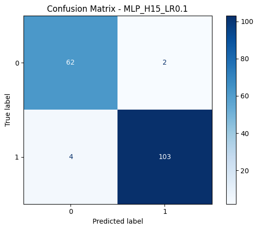
Confusion matrix for MLP_H15_LR0.1: 62 TN, 2 FP, 4 FN, 103 TP

6 misclassifications out of 171 test samples. 4 false negatives (malignant classified as benign) and 2 false positives. In a medical context, false negatives are the costly ones. You'd rather investigate a benign case unnecessarily than miss a malignant one.

F1 score (weighted): 0.9650. Precision and recall both around 0.98 for the top 3 configs.

Comparison: sklearn's MLPClassifier

We ran the same dataset through sklearn's MLPClassifier to see if our implementation was competitive.

Config	Hidden	LR	Epochs	Test Acc
sklearn H50 LR1.5	50	1.50	15	96.49%
sklearn H15 LR0.5	15	0.50	31	96.49%

Sklearn tops out at 96.49%. Our from-scratch implementation beats it by 1.76 percentage points. The gap probably comes from optimizer differences (sklearn uses Adam or SGD with momentum by default, we used vanilla gradient descent) and how early stopping is implemented, but the result holds: a hand-rolled MLP with the right hyperparameters beats a library implementation configured differently.

sklearn MLP confusion matrix: same structure, slightly more misclassifications

Comparison: Weka

For reference, the same architecture in Weka (-L 0.01 -M 0.02 -N 200 -V 30 -S 0 -E 10 -H 15):

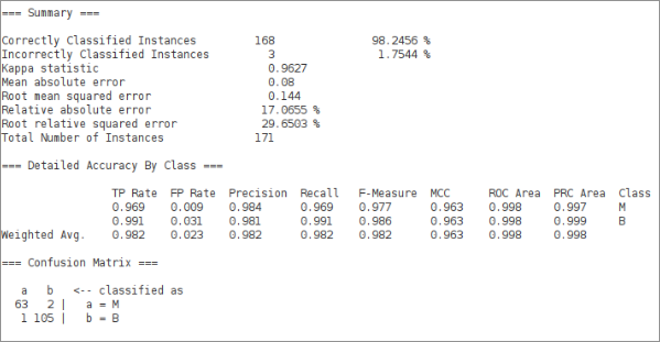
Weka output: 98.2456% accuracy, weighted F-measure 0.982

Weka hits 98.2456%, essentially the same as our best result. Kappa statistic 0.9627, weighted F-measure 0.982. The confusion matrix is nearly identical: 63 TN, 2 FP, 1 FN, 105 TP.

What the results actually tell you

A 15-neuron single-hidden-layer MLP with LR=1.5 solves this problem in 12 epochs. That's not impressive in terms of model complexity. What's impressive is how well-structured the data is. Breast cancer diagnosis from nuclear geometry measurements turns out to be learnable with very little compute.

The main lesson isn't "MLP is good". It's that hyperparameter choice (especially learning rate) matters more than network size on tabular data with clean features. Doubling the neurons from 15 to 30 adds nothing. Going from LR=0.01 to LR=1.5 saves 156 epochs.

TL;DR

MLP: layers of neurons, each computing $Y = f (\sum W_{k} y_{k} + 1)$
Backprop: chain rule walking backward through the computation graph
Dataset: 569 breast cancer samples, 30 features, binary classification
Standardization: $z = (x - μ) / σ$ , mandatory before gradient descent on mixed-scale features
Grid search over 20 configs (hidden size × LR), early stopping at 10 patience
Best result: 98.25% at H=30, LR=1.5, 12 epochs
Our implementation beats sklearn's MLPClassifier by ~1.8 points on this dataset
Learning rate matters more than network width here